Recurrent Neural Networks (RNNs): Teaching AI to Understand Sequences 🔁🧠

Introduction 🌱

Imagine listening to a song and predicting the next note, or reading a sentence and anticipating the next word. Our brains excel at understanding sequences because they remember previous elements. Recurrent Neural Networks (RNNs) enable AI to do the same—processing sequential data like speech, text, and time series. This article explores how RNNs work, their structure, applications, and why they’re essential for tasks involving sequences.

What Are Recurrent Neural Networks (RNNs)? 🤔

RNNs are a type of neural network designed to process sequential data by maintaining a memory of previous inputs. Unlike traditional neural networks that treat each input independently, RNNs have loops that allow information to persist. This memory makes them ideal for tasks like language modeling, speech recognition, and stock price prediction.

Key components of an RNN include:

• Neurons (Nodes) 🧩: Units that receive and process information.
• Hidden States 💾: Internal memory that stores information from previous inputs.
• Weights ⚖️: Parameters that determine the importance of each input.
• Activation Functions 🚦: Functions that introduce non-linearity, enabling the network to learn complex patterns.

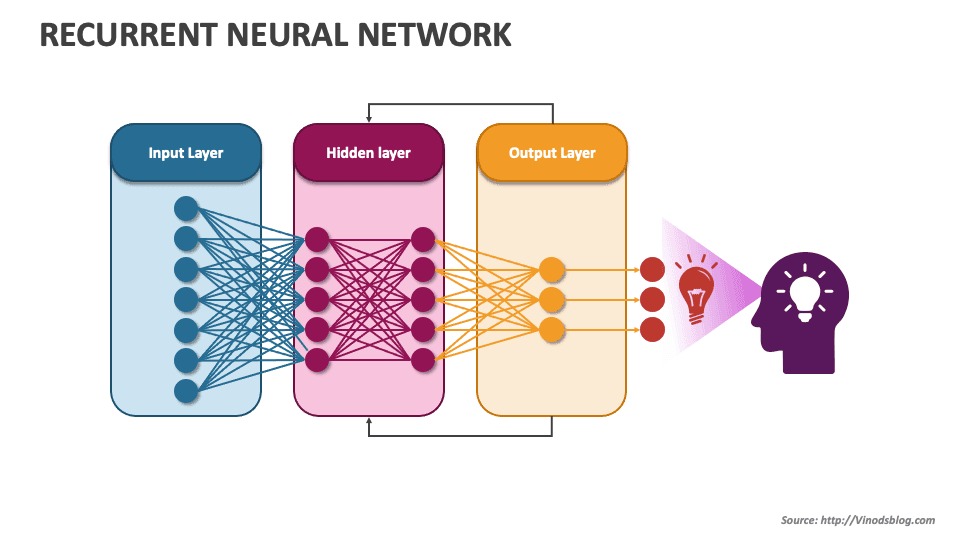
How RNNs Work: Step-by-Step Process ⚙️

RNNs process data sequentially, one element at a time, while maintaining a hidden state that captures information from previous elements. Here’s how the process works:

1. Input Layer 🟢:
   The network receives a sequence of data (e.g., a sentence or time series). Each element is fed into the network one by one.

2. Hidden Layer 🔄:
   At each step, the neuron processes the current input and the hidden state from the previous step, generating a new hidden state. This allows the network to remember information from earlier inputs.

3. Output Layer 🎯:
   The final output is generated based on the hidden state at the last step, or at each step if the task requires predictions for every element in the sequence.

4. Loop Structure ♻️:
   The loop in the hidden layer allows information to be passed from one step to the next, creating a temporal memory that captures patterns across the sequence.

Mathematical Representation 🧮

At each time step $t$, the RNN performs the following calculations:

• Hidden state:

ht=tanh⁡(Whxxt+Whhht−1+bh)h_t = \tanh(W_{hx}x_t + W_{hh}h_{t-1} + b_h)ht​=tanh(Whx​xt​+Whh​ht−1​+bh​)

• Output:

yt=Whyht+byy_t = W_{hy}h_t + b_yyt​=Why​ht​+by​

Where:

• xtx_txt​ is the input at time step $t$.
• hth_tht​ is the hidden state at time step $t$.
• Whx,Whh,WhyW_{hx}, W_{hh}, W_{hy}Whx​,Whh​,Why​ are weight matrices.
• bh,byb_h, b_ybh​,by​ are bias terms.
• $\tanh$ is the activation function, which adds non-linearity.

Training RNNs: Learning From Sequences 📚

Training an RNN involves adjusting its weights to minimize prediction errors using a process called Backpropagation Through Time (BPTT). This method is similar to standard backpropagation but considers the sequential nature of the data.

1. Forward Propagation 🏹:
   The network processes the entire sequence, generating hidden states and outputs at each step.

2. Loss Calculation 💡:
   The network compares its predictions to the actual outputs using a loss function (e.g., cross-entropy for classification or mean squared error for regression).

3. Backward Propagation Through Time (BPTT) 🔁:
   The network calculates gradients by unfolding the sequence and applying backpropagation to each step.

4. Weight Update ⚖️:
   The network adjusts its weights using optimization algorithms like Stochastic Gradient Descent (SGD) or Adam.

Challenges of RNNs: Vanishing and Exploding Gradients ⚠️

RNNs face two key challenges when processing long sequences:

• Vanishing Gradient Problem:
  Gradients become very small during backpropagation, making it difficult for the network to learn long-term dependencies.

• Exploding Gradient Problem:
  Gradients become excessively large, causing unstable updates and poor convergence.

To address these issues, advanced architectures like Long Short-Term Memory (LSTM) and Gated Recurrent Units (GRU) were developed.

Advanced RNN Architectures 🏗️

1. Long Short-Term Memory (LSTM) 🧠

LSTMs use special memory cells and gates (input, forget, and output gates) to regulate the flow of information. This design helps LSTMs maintain long-term dependencies without suffering from vanishing gradients.

2. Gated Recurrent Unit (GRU) 🔄

GRUs are similar to LSTMs but have a simpler structure with fewer gates, making them more computationally efficient. Despite their simplicity, GRUs often perform as well as LSTMs on many tasks.

Real-World Applications of RNNs 🌍

• Natural Language Processing (NLP) 💬:

  • Language modeling, text generation, and machine translation.
  • Chatbots that understand and respond to user queries.

• Speech Recognition 🎙️:

  • Converting spoken language into text (e.g., virtual assistants like Siri and Alexa).

• Time Series Forecasting 📊:

  • Predicting stock prices, weather patterns, and energy consumption.

• Video Analysis 📹:

  • Recognizing actions and events in video sequences.

• Healthcare 🏥:

  • Analyzing patient data to predict disease progression.

Building a Sequence Classifier Using RNN 🏗️

1. Data Collection and Preprocessing 🗂️🧹

• Collect sequential data (e.g., text, audio, or time series).
• Tokenize and normalize the data for consistency.

2. Designing the RNN Architecture 🏗️

• Input layer: Accepts sequential data.
• Hidden layers: Maintain hidden states to capture temporal patterns.
• Output layer: Generates predictions based on the final hidden state.

3. Training the RNN 📚🏹

• Train the network using BPTT and optimize weights using algorithms like Adam or RMSprop.
• Use regularization techniques like dropout to prevent overfitting.

4. Evaluating the RNN 📊

• Assess performance using metrics like accuracy, precision, recall, and F1-score.
• Fine-tune the network to improve generalization.

5. Testing and Deployment 🚀

• Test the trained RNN on unseen sequences to evaluate its real-world performance.
• Deploy the model for practical applications like language translation or stock price prediction.

Advantages and Limitations ⚖️

✅ Advantages:

• Captures temporal dependencies in sequential data.
• Processes variable-length sequences without fixed-size input.
• Handles both short-term and long-term patterns (with LSTM/GRU).

❗ Limitations:

• Struggles with very long sequences due to vanishing gradients.
• Slower training due to sequential processing.
• Limited scalability compared to transformer models like GPT and BERT.

The Future of RNNs 🚀

While RNNs have paved the way for sequence modeling, newer architectures like Transformers are now dominating NLP and time series tasks. However, RNNs—especially LSTMs and GRUs—remain valuable for applications requiring compact models with temporal memory. As AI continues to evolve, RNNs will likely play a supporting role in hybrid systems that combine their strengths with advanced architectures.

Conclusion 🌟

Recurrent Neural Networks have transformed AI’s ability to understand and process sequential data, enabling breakthroughs in speech recognition, language translation, and time series forecasting. By capturing temporal dependencies and maintaining memory, RNNs mimic the human brain’s ability to understand sequences. As technology advances, RNNs will continue to shape the future of AI applications that rely on sequential information.